Because of the risk of this, if this is new we are likely to advise you to attend hospital. We may advise you to attend a specialist cardiac hospital, depending on your symptoms and other signs of illness that you might have called us for. If you already know you have the condition, it is worth noting it down and keeping a copy of your ECG trace for any future queries.
If you are a healthcare professional and you are reading this, please let us know what you think by commenting or getting in touch. Would you use this to explain the condition to your patients?
Often basic ECG teaching relies on teaching pattern recognition, which can work well, however when presented with an ECG that isn’t similar to a pattern you have seen, you can run in to problems.
This article will explore two simple concepts that will hopefully help with your ECG reading and understanding of the underlying physiology:
It can be good to think of an ECG as a graph with an X and Y axis. X, horizontally along the bottom represents time. We’ll come to the Y axis later.
Now, we know that X is time, each small square is 40ms (0.04seconds), each large square is 200ms (0.2 seconds), 30 large squares is 6 seconds and so on. That’s reasonably straightforward, but how does it relate to physiology?
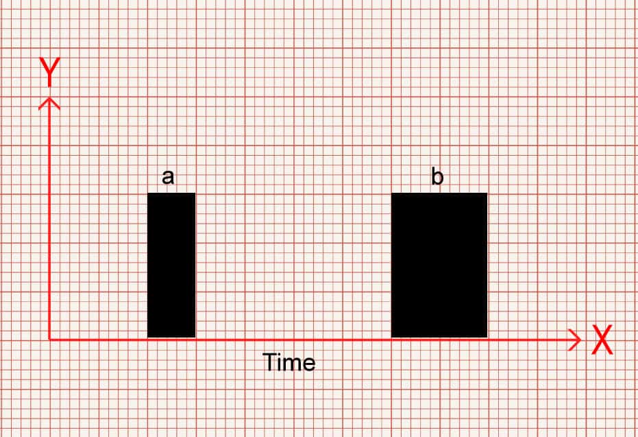
Let’s imagine that graph again. And let’s imagine some boxes drawn on. Don’t worry about the Y axis value for now.
In image 1 you can see a narrow box (a) and a wider box (b). Which one would you say takes up more time? Which one takes up less time?
Box b takes up more of space along the X axis so therefore takes up more time. Box a covers less space on the X axis so takes less time.
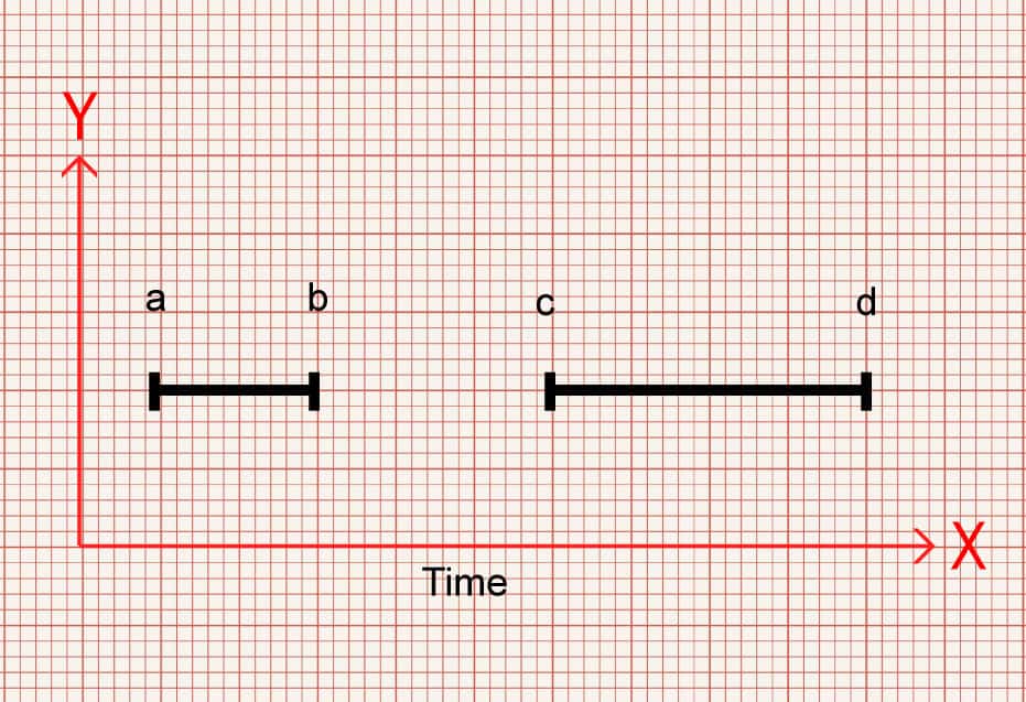
Similarly, we can measure between two points. Look at Image 2. You can see two horizontal lines of different lengths. The gap between a – b is shorter than c -d. So again, which takes up more time?
Gap c-d is wider, takes up more of the X axis and therefore takes up more time.
Stay with me.
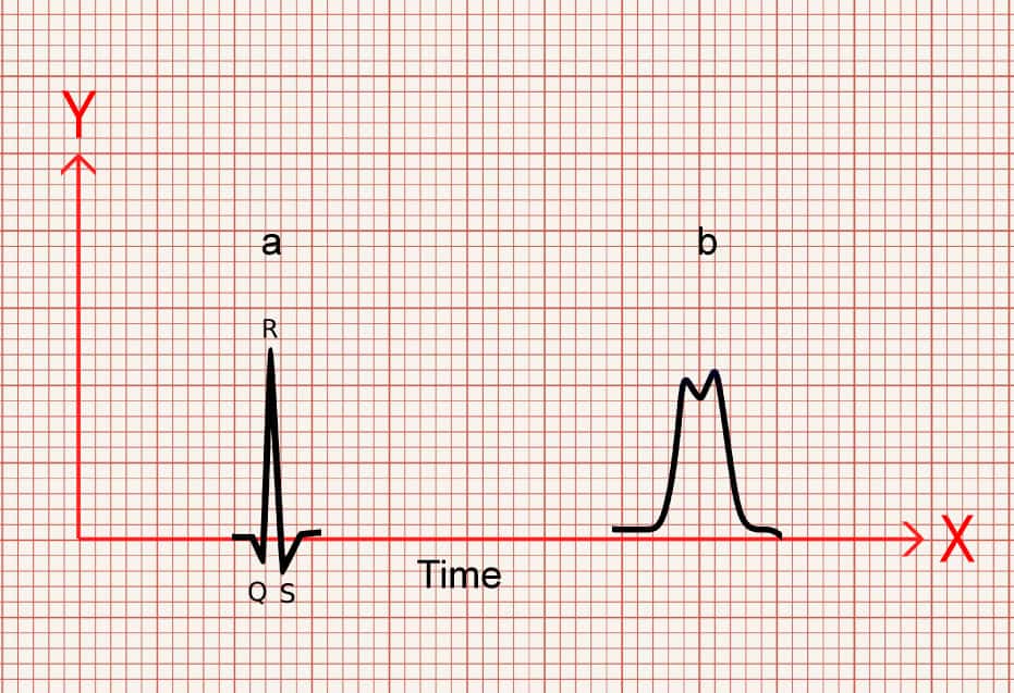
Now, let’s replace those boxes with QRS complexes.
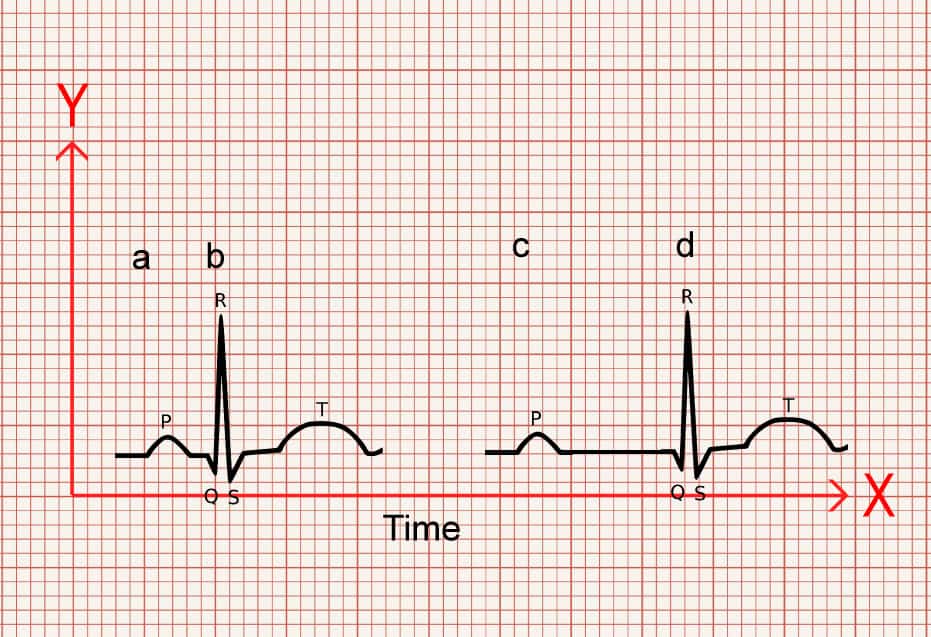
In image 3 there is a narrow QRS (a) and a wider QRS (b). Which one takes up more time?
B is taking up more of the X axis so takes more time.
And again, once more, let’s look at some gaps between two points, but let’s show it as the gap between the P wave and QRS. Which one takes up more time and which takes up less time?
The gap between a-b is shorter than c-d.
So c-d takes up more time.
Probably not ground breaking.
But, what’s another way of thinking about the time something takes? If something takes up more time, you could also say that it is slower, and if something takes up less time, its faster.
Now, remember that an ECG is dealing with electrical conduction.
If on an ECG something is taking up more space along the X axis, therefore taking more time, and is therefore slower, then it makes sense that there is a problem effecting its ability to conduct!
And poor conduction is the underlying issue that what we see in AV blocks and bundle branch blocks.
So if you see a QRS or PR that is wider than normal values, think, something is causing it to be slower and that there is a conduction fault.
Equally if you see a PR interval that is narrower than it is meant to be, taking up less space along the x axis and therefore less time, think, it’s conducting faster than it should and it would alert you to pre-excitation problems, such as accessory pathways in Wolff-Parkinson-White syndrome (WPW effects both the PR interval making it shorter, and has a wider QRS).
Direction
Now, let’s talk about direction.
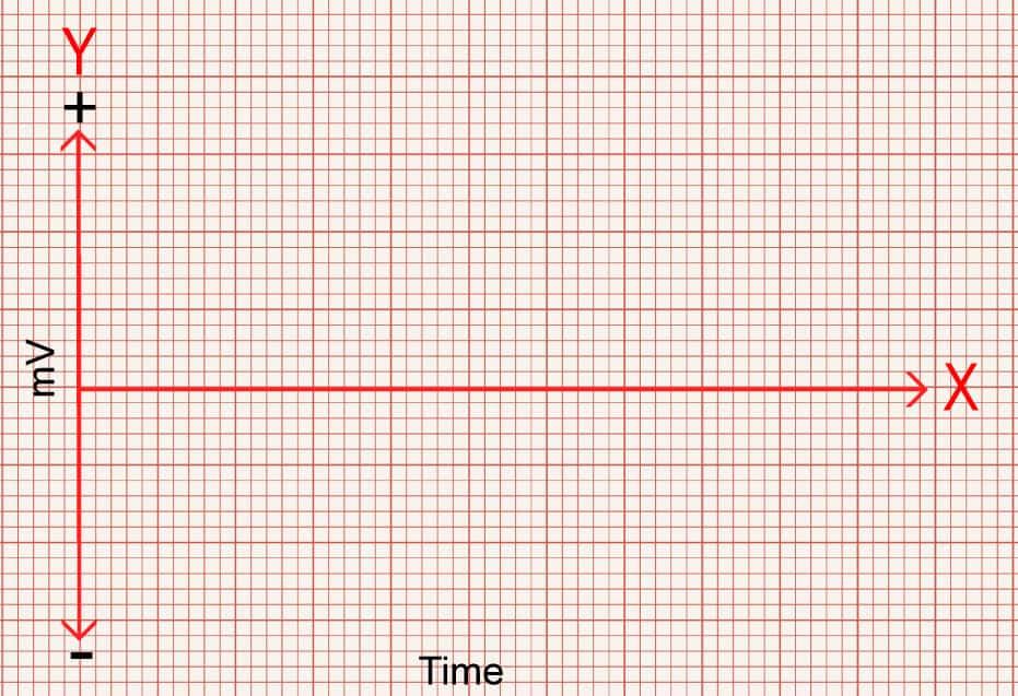
We know by looking at the ECG paper that vertically, the small boxes, measured in mm, represent millivolts (mV) – a measure of force (sort of). Each 1mm = 0.1mV, 10mm = 1mV. This also means that it has what’s known as magnitude – or size.
Now, let’s look at the graph again. We know the X axis is time, as discussed above. However, in an ECG the X axis is not simply the bottom, but instead the middle of the graph, with the Y axis extending both positively above the X, and negatively below the X axis.
The X axis can have readings above or below it. This is the isoelectric line.
ECGs pick up electrical charge moving across the heart. And it does so by placing electrodes at different locations around the heart.
As shown in the diagram below, the electrodes create a view of the heart from different angles, and each view is called a lead. 12 leads (views), but only 10 wires.
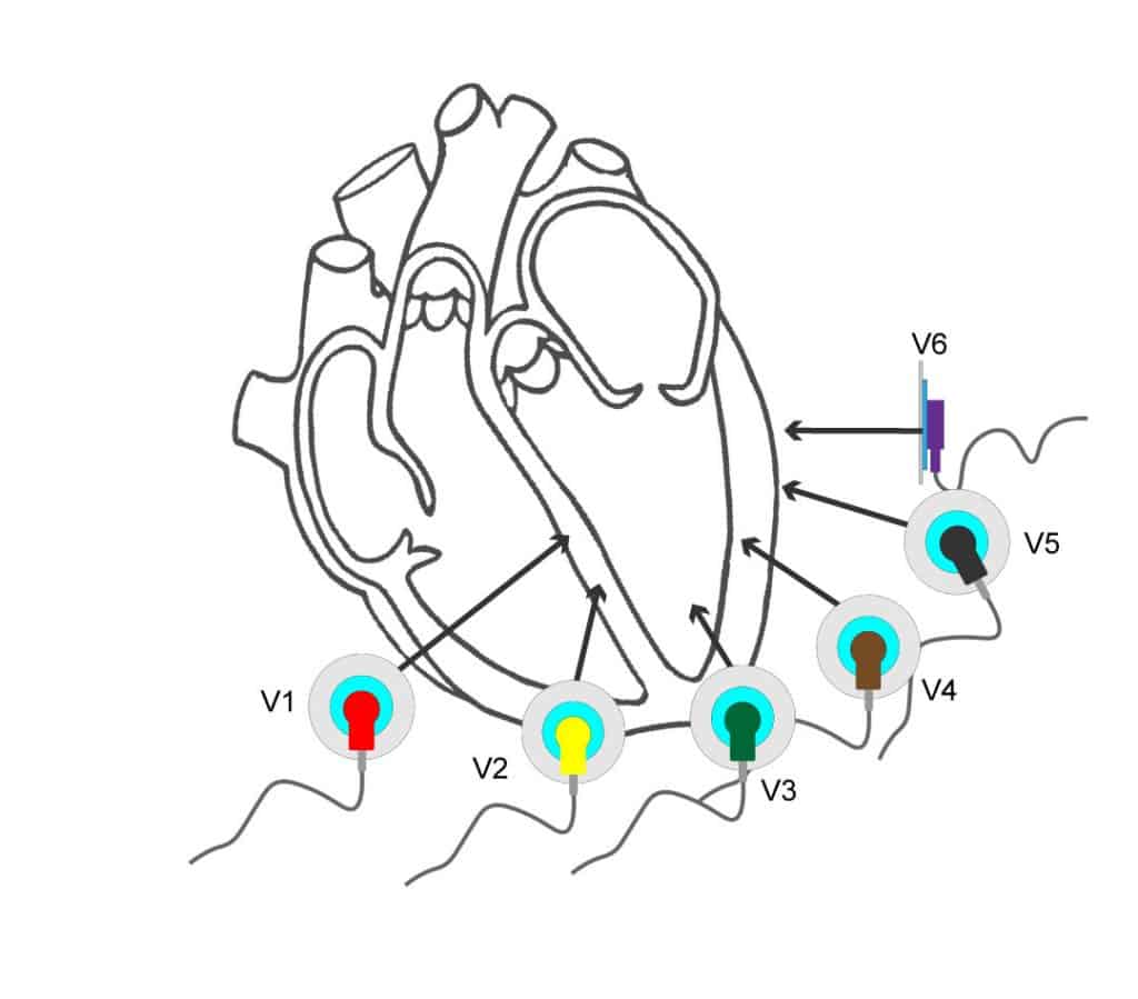
The chest leads look at the heart across the transverse plane, that is from the front of the chest to the back, whereas the limb leads look at the heart in the frontal plane, which are essentially from the sides, top and bottom.
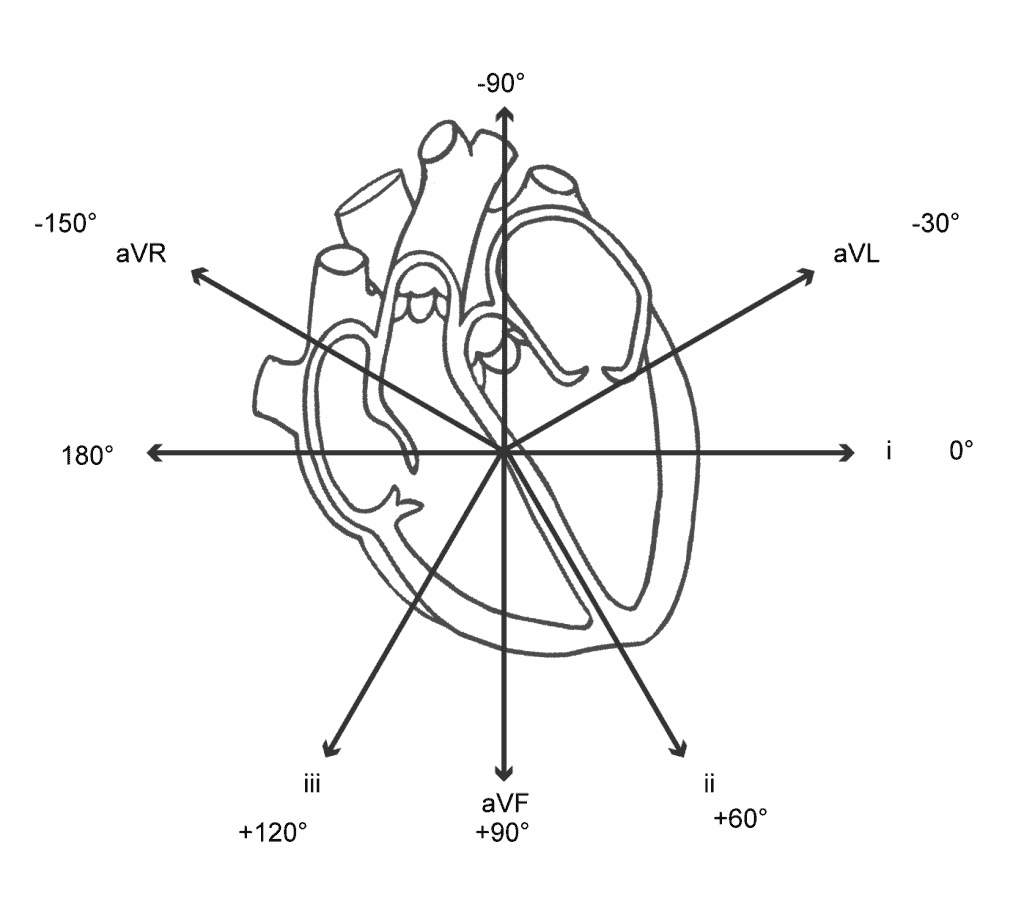
The angles the leads look at the heart are measured in degrees, with lead i being the reference point of 0°.
This is something that is worth learning so that you are able to visualise where each lead “looks”.
Roughly speaking, the limbs leads create the following views of the heart.
avR – Looks from the Right shoulder to the left hip
aVL – Looks from Left shoulder to right hip
i – Looks from the left mid axilla similar to V6
ii – Looks from the left hip to right shoulder
aVF – Looks from the Feet up to the head
iii – Looks from the right hip to the left shoulder
The chest leads create views from the chest wall through to the back
V1 + V2 – intraventricular septum
V3 – V4 – anterior wall of the left ventricle
V5 – V6 – lateral wall of the left ventricle
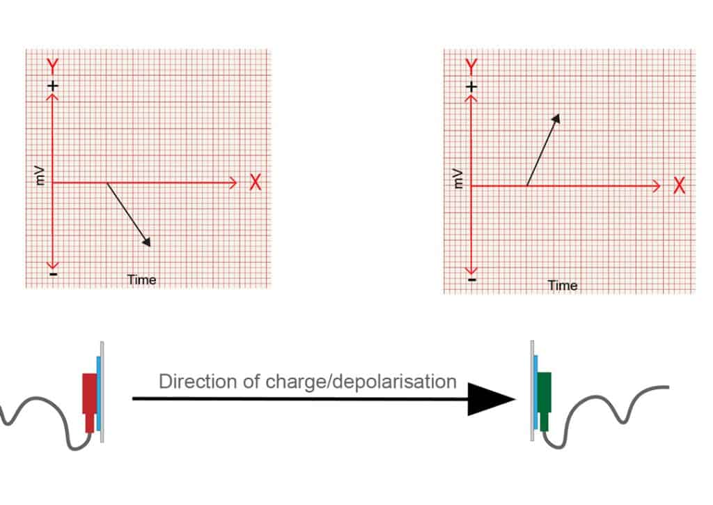
Very simply put, as an electrical charge moves towards an electrode position, this creates a positive reading. As it moves away it creates a negative reading.
Electrodes that are opposite to each other, 180 degrees apart, will be mirrored. One will have charge moving towards it, creating a positive deflection and the opposite side will show a negative deflection as the charge moves away from it.
Leads at 180° from each other.
Slightly more complicated is what happens when the electrical charge isn’t moving directly to, or away from the electrode, but when it is moving at more or less than 180 degrees to the electrodes position.
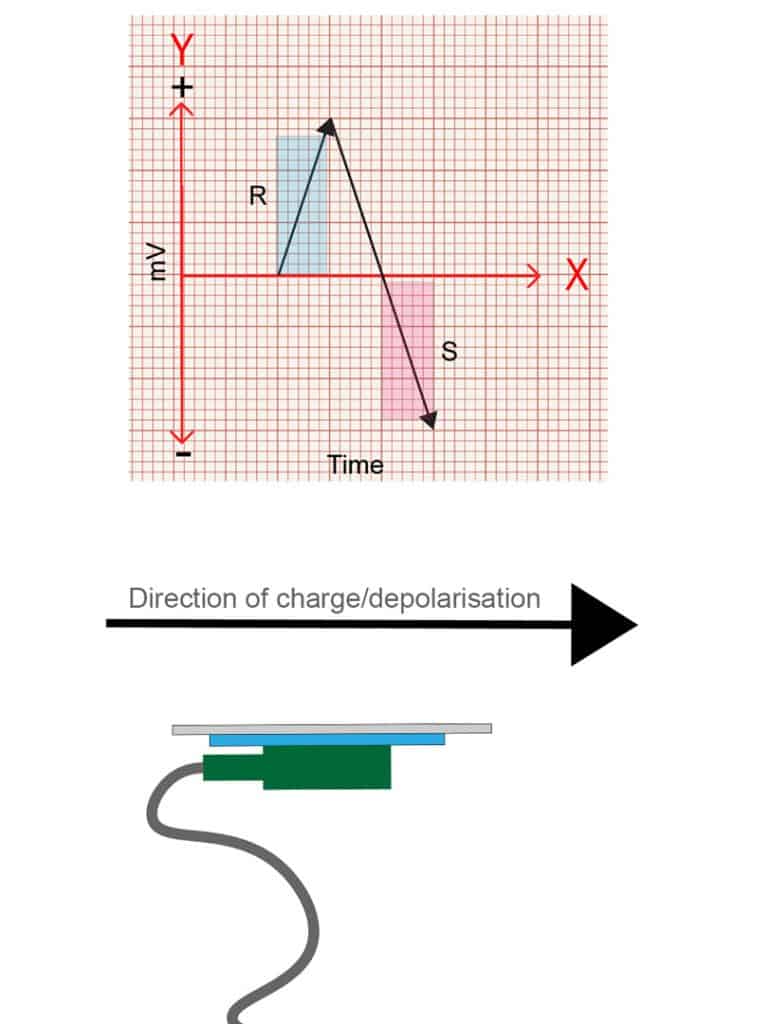
Let’s look at what happens when it moves at 90 degrees to the electrode first.
When the charge is moving at 90 degrees, or perpendicular, to the position of the electrode, it has both a period of positivity and a period of negativity, as the charge moves towards and then away from the electrodes position as it passes by. This is represented on an ECG as an R wave followed by an S wave of equal magnitude.
Quick tip – an R wave is any positive deflection you see, and an S wave is a negative deflection following an R wave BUT it must cross the isoelectric line to be considered negative. The segment from the top of the R wave back to the isoelectric line is not the S wave. The S wave is only the portion below the isoelectric line.
Hopefully this is starting show the relationship between the direction of the charge and the position of the electrode.
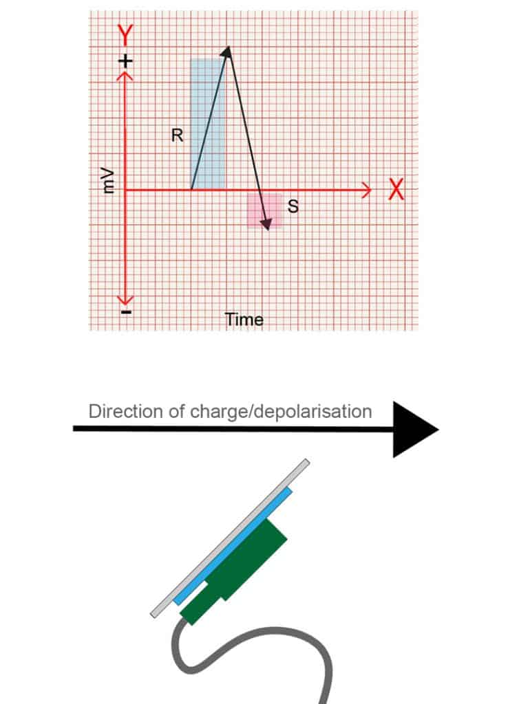
So, what happens if the charge moves at 45 degrees to an electrode’s position? Well, it’s a bit more towards the electrode than 90 degrees, but not straight on. So the tracing will show a predominately positive wave, with a smaller S wave. The opposite will be true if travelling at say 135 degrees away from an electrode.
Hopefully you can see then, that by varying the direction the charge travels, you’ll get different combinations of positive and negative deflections, and that it is relative to the position of each lead/view!
This means that the waves on an ECG not only have a value in magnitude (mV), but also direction. This combination of magnitude and direction is known as a vector.
So not only can the ECG waves tell you the charge in volts, but it can also show you the direction that charge is moving relative to the electrode placement.
Why is this important?
Well, many of the pathologies we come across effect the direction the charge moves across the heart.
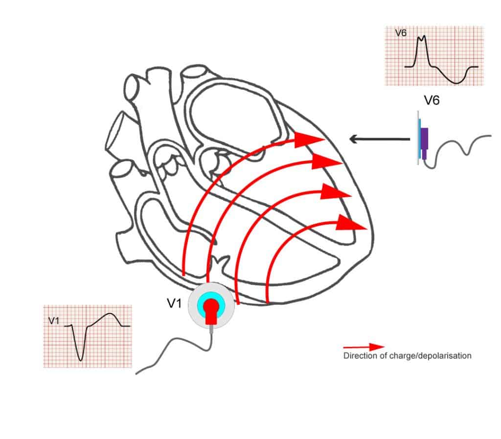
For example, in left bundle branch block (LBBB), the left conduction pathway is faulty. This means all of the electrical charge must come from the right side of the heart, and travels across the heart from right to left through the slower conducting muscle tissue.
V1 looks at the right side of the heart, so, with right to left movement, the charge is moving , slowly, away from V1, giving the classic negative, deep S wave seen in LBBB.
Understanding the concepts of vectors is important if you want to understand axis deviation, reciprocal changes in STEMIs, left anterior and left posterior fascicular blocks, T wave inversions and strain patterns, and how to identify bundle branch blocks.
Final Notes
So, to sum up, understanding how time is displayed on the ECG will lead to better recognition of conduction faults. Understanding that the ECG shows both direction and magnitude means you can easily understand how that charge is moving across the heart. Couple this with further reading around the physiology and pathophysiology and your ECG interpretation should greatly improve!
Just as a final caveat: electrophysiology is complicated. This is a basic description of the principles and vectors, but the images are not exact examples. The detailed process of how the electrodes work, how the leads form their views, the physics behind it and so on are far beyond the scope of this article, but hopefully this has given some insight into the applied nature of ECG.
References
The above post is written by an Article999 contributor and contains a mix of original content and explanations based on the below sources. All images are combined from licensed Adobe Stock images and the author’s own work, as with all Article999 content.